How to define Solid Boundary Conditions in Local Base (defined by vector)
Go to FE Model\Boundary Conditions\Solid BC\On node choose X direction, select Local base and press Define local base button.
In Local base dialog box choose Vector and enter vector coordinates.
Use Get defined vector button when vector was defined by picking face/edge or were defined by another graphical tool.


How to define Solid Boundary Conditions in Cylindrical Local Base
How to use Data Super Elements to set spatial variations of material properties
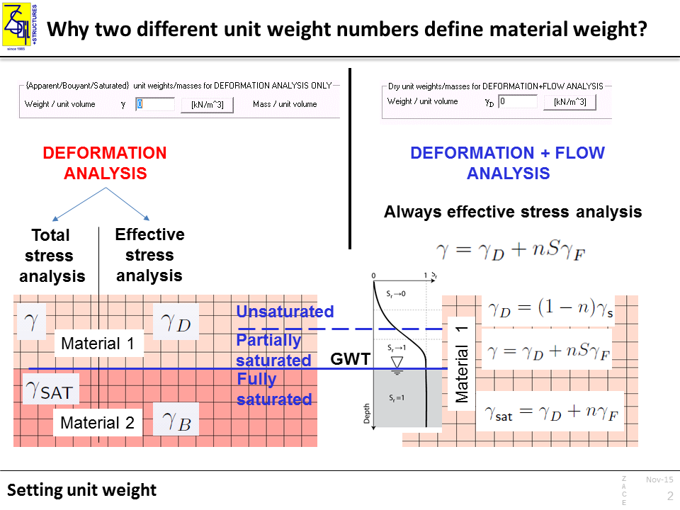
Why two different unit weight numbers define material weight?
Two different unit weights define material weight for two different types of numerical analysis:
1. Deformation analysis for which material is considered as a single-phase medium
2. Deformation + Flow analysis where material is a double-phase medium which consists of skeleton and fluid that fills voids

The Deformation + Flow analysis is always considered as the effective stress analysis. In this case, material consists of skeleton and voids which can be filled with water.
Therefore, an apparent weight of each finite element depends on unit weight of dry material gD, its current porosity n, and the saturation degree S. It means that the weight may vary for the same material depending on saturation conditions.
In the case of Deformation analysis (single-phase continuum), material’s weight remains constant throughout the entire simulation. If the material is considered as a solid-fluid mixture, one has to decide which type of analysis is intended to be carried out:
1 . Total stress analysis – used when modelling undrained behavior using total stress parameters, e.g. φ = 0, c = Su (undrained shear strength)
or
2. Effective stress analysis – using effective stress parameters and assuming free drainage conditions in the real conditions.
In both cases, a ground water table (GWT), if such exists, should be taken into account. Therefore, geotechnical layer should be discretized in the model with the aid of two different materials although they share the same mechanical parameters.
The following unit weights can be assumed:
1.Total stress analysis – unit weight of soil with natural moisture γ above GWT, and unit weight of saturated soil γSAT below GWT
2.Effective stress analysis – unit weight of dry soil, γD, should be given to compute the profile of effective stresses above GWT, whereas buoyant weight of soil γB = γSAT – γF should be defined for the fully saturated soil
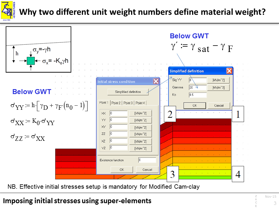
In some cases the initial stress can be imposed by the user be means of so-called super-elements.
Imposing initial stresses can solve convergence issues in the case of the boundary value problems that include construction works, e.g. an embankment. The initial stresses should be then imposed on the introduced finite elements. Imposing initial stresses is mandatory for the Modified Cam-clay model since the initial shear modulus is computed based on the mean effective stress.
Initial stresses super-elements can be defined in PreProcessor (Initial Conditions -> Initial Stresses), by selecting 4 nodes (2D) or 8 nodes (3D) . Note that the compressive stresses are negative numbers. In the case of Deformation+Flow analysis the imposed initial stresses always define effective stresses.
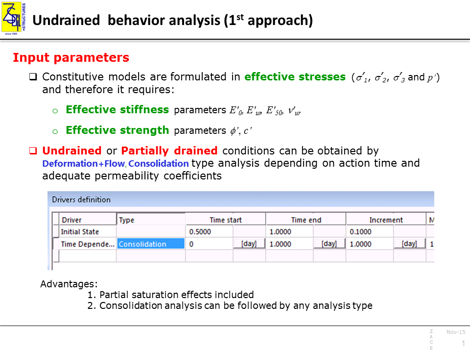
How to simulate the undrained behavior?
Simulating the undrained behavior of soil can be carried out by means of three different approaches:
- Effective stress analysis using Consolidation driver type for Deformation+Flow problem type
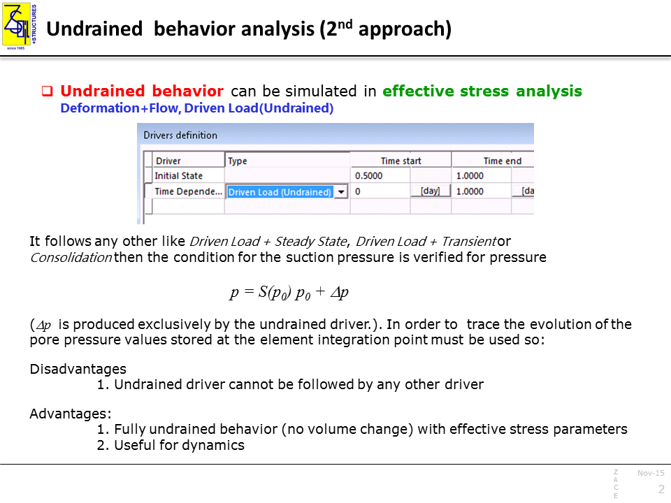
- Effective stress analysis using Driven Load-Undrained driver type for Deformation+Flow problem type
- Total stress analysis using Driven Load driver type for single-phase Deformation problem type
These approaches are described below.
CONSOLIDATION
Driver setup: Deformation+Flow, Time Dependent, Consolidation
Input parameters: always effective strength and stiffness parameters
Advantages:
- undrained or partially drained conditions arise naturally depending on action time and soil permeability
- partial saturation effects are included
- consolidation analysis can be followed by any analysis type
Disadvantages:
- CPU time for very large boundary value problems
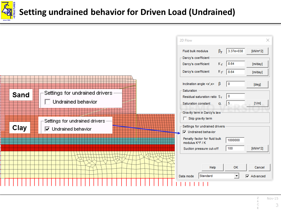
DRIVEN LOAD – UNDRAINED
Driver setup: Deformation+Flow, Time Dependent, Driven Load (Undrained)
Input parameters: effective strength and stiffness parameters
Advantages:
- fully undrained regime (no volume change) is obtained regardless defined soil soil permeability
- useful for dynamics
Disadvantages:
- Undrained driver cannot be followed by any other driver
Using Undrained driver type, special attention must be paid on appropriate selection of undrained driver settings. Undrained behavior can be disabled for material layers for which undrained behavior is not relevant.
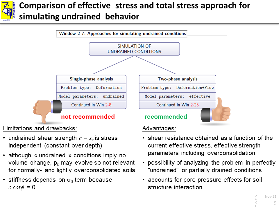
TOTAL STRESS ANALYSIS
Driver setup: Deformation, Time Dependent, Driven Load
Input parameters: total stress strength and stiffness parameters
Advantages:
- relatively fast in terms of CPU
Disadvantages:
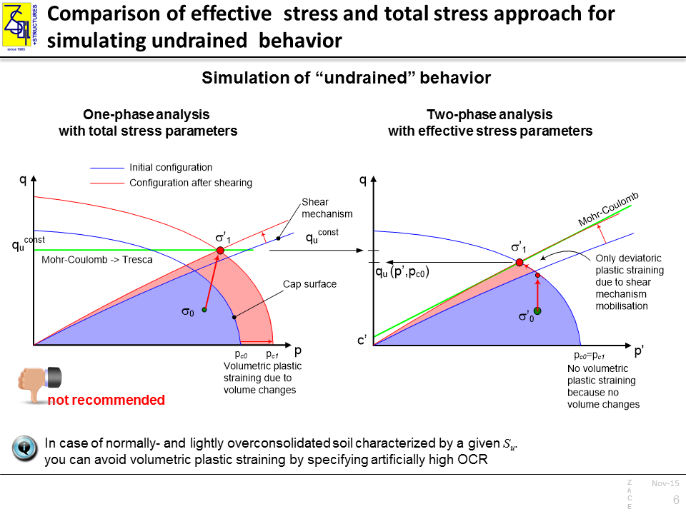
- undrained shear strength c = Su is stress independent (i.e. constant over depth; typically, not the case in natural conditions)
- although « undrained » conditions imply no volume change, model’s preconsolidation pressure pc may evolve so not relevant for normally- and lightly overconsolidated soils
- stiffness depends on φc term because c cot φ = 0
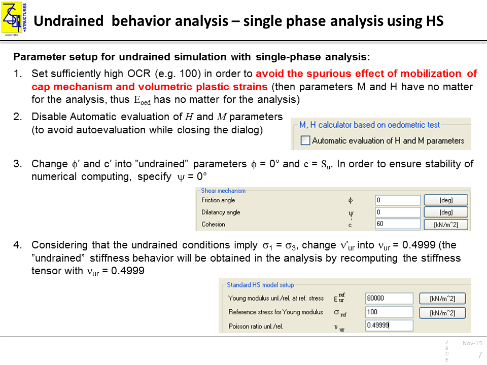
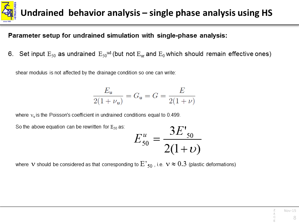
The use of the Hardening-Soil model to simulate undrained behavior with the total stress approach demands the parameter setup which presented below.
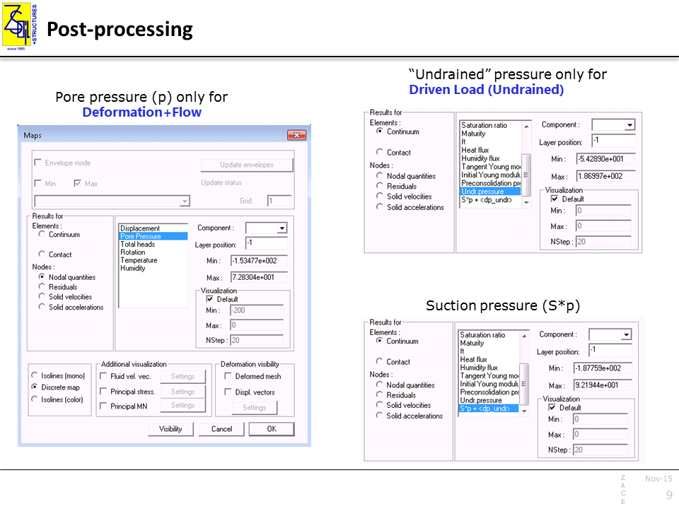
POST-PROCESSING
Pore pressure
For Consolidation analysis, pore pressure values can be standardily visualized using nodal quantities. In the case of Undrained driver, the results are stored in the Gauss points and visualization of pore pressure can be done using “Undrained pressure” under continuum element results.
Suction pressure (S*p)
Magnitudes of suction pressure are stored in the Gauss points and can be read using S*p + <dp_undr> under continuum element results.